D-Claw modeling of the 2014, Oso, Washington landslide disaster reveals potential mobility bifurcations due to initial material parameters.
This page features material and excerpts from:
Landslides that liquefy: modeling mobility bifurcation and the 2014 Oso, Washington, USA disaster. R.M. Iverson, D.L. George, 2016. Geotechnique, V. 66(3), 175–187. pdf
see also:
Landslide mobility and hazards: implications of the 2014 Oso disaster. R.M. Iverson, D.L. George, et al., 2015. Earth Planet. Sci. Lett., V. 412, pp. 197–208. pdf
Abstract
Some landslides move slowly or intermittently downslope, but others liquefy during the early stages of motion, leading to runaway acceleration and high-speed runout across low-relief terrain. Mechanisms responsible for this disparate behaviour are represented in a two-phase, depth-integrated, landslide dynamics model that melds principles from soil mechanics, granular mechanics and fluid mechanics. The model assumes that gradually increasing pore-water pressure causes slope failure to nucleate at the weakest point on a basal slip surface in a statically balanced mass. Failure then spreads to adjacent regions as a result of momentum exchange. Liquefaction is contingent on pore-pressure feedback that depends on the initial soil state. The importance of this feedback is illustrated by using the model to study the dynamics of a disastrous landslide that occurred near Oso, Washington, USA, on 22 March 2014. Alternative simulations of the event reveal the pronounced effects of a landslide mobility bifurcation that occurs if the initial void ratio of water-saturated soil equals the lithostatic, critical-state void ratio. They also show that the tendency for bifurcation increases as the soil permeability decreases. The bifurcation implies that it can be difficult to discriminate conditions that favour slow landsliding from those that favour liquefaction and long runout.
D-Claw modeling of landslide dynamics at Oso
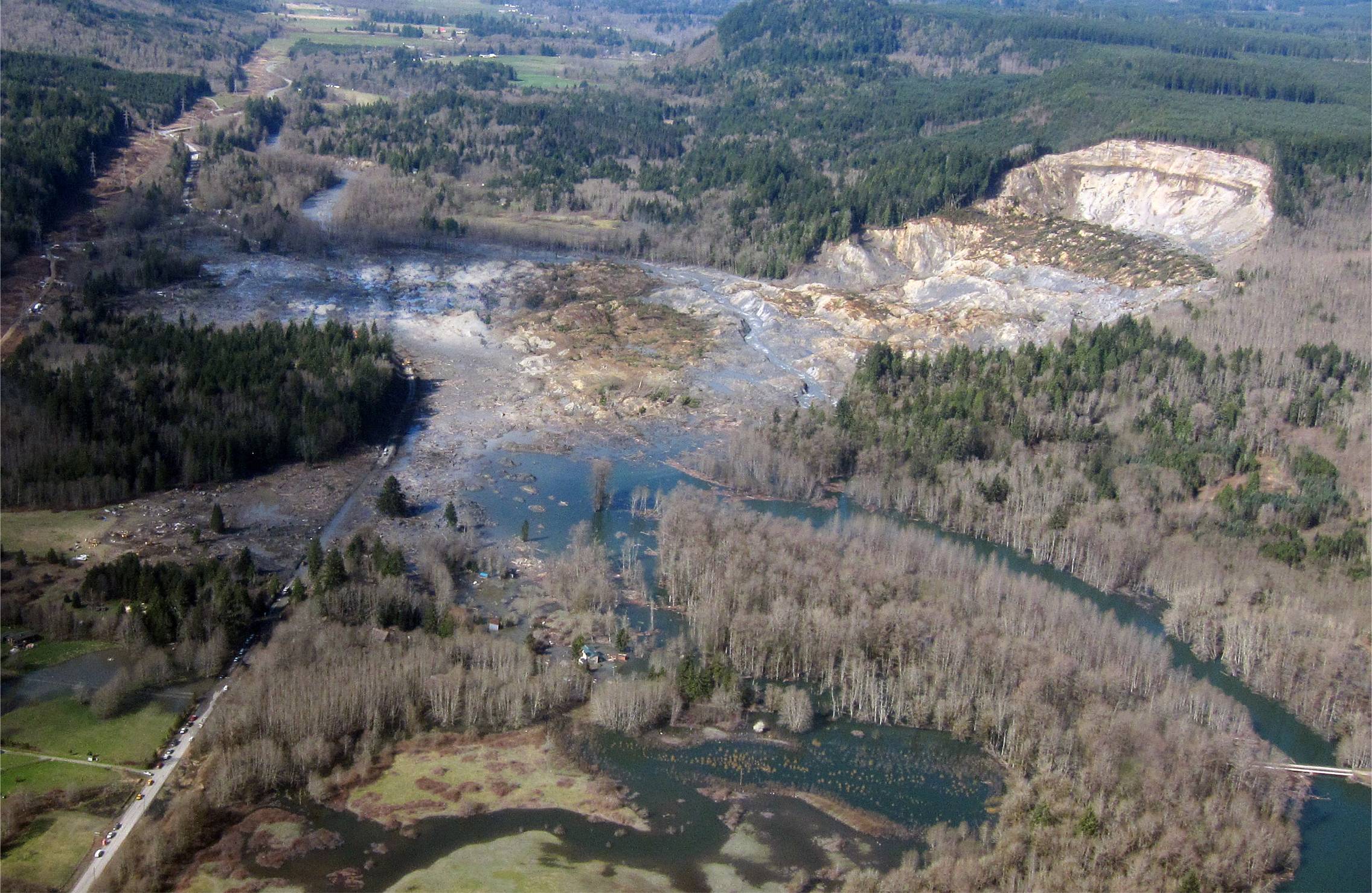
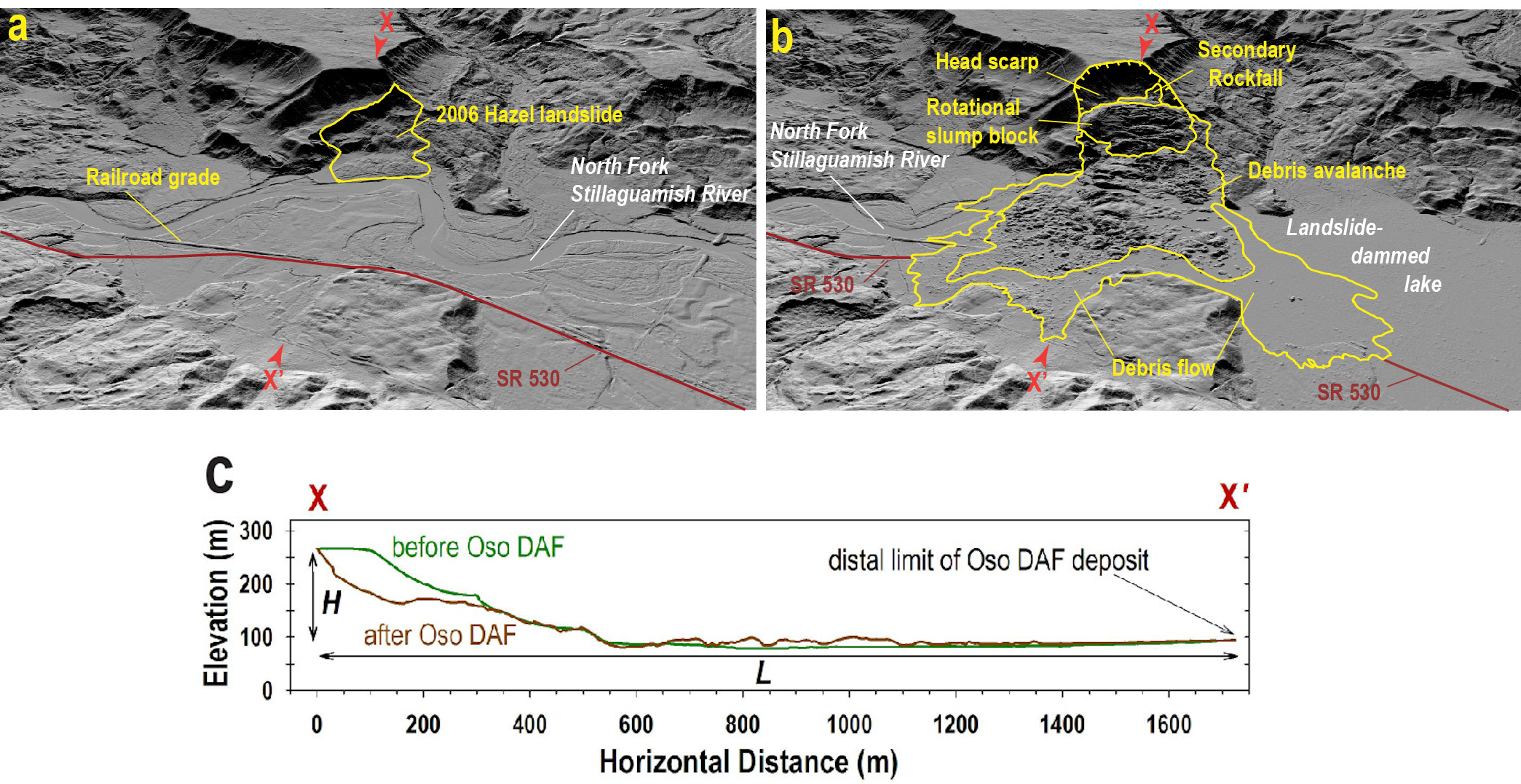
D-Claw is used to study the dynamics of a large, high mobility landslide that occurred following a long period of unusually wet weather near Oso, Washington, USA, on 22 March 2014. The landslide (officially named the SR 530 landslide by Washington State) caused 43 fatalities, ranking it second only to a 1985 event in Mameyes, Puerto Rico, as the worst landslide disaster in US history (cf. Jibson, 1992). Results of a multidisciplinary investigation of the landslide’s behaviour are presented elsewhere (Iverson et al., 2015).
D-Claw considers the gravity driven motion of fluid-filled granular mixtures that can undergo dilation and contraction during both quasi-static and inertial deformation. The model employs depth integrated continuum mechanical equations that blend concepts from critical-state soil mechanics, fluid mechanics and granular mechanics. Iverson & George (2014) provide a comprehensive derivation of the model equations, and George & Iverson (2014) describe the numerical method of solving the equations, as well as tests of model predictions against data from large-scale experiments.
Landslide source initialization for D-Claw modeling
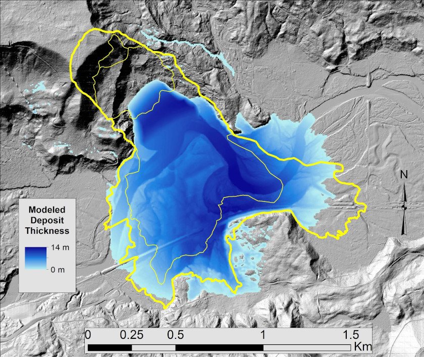
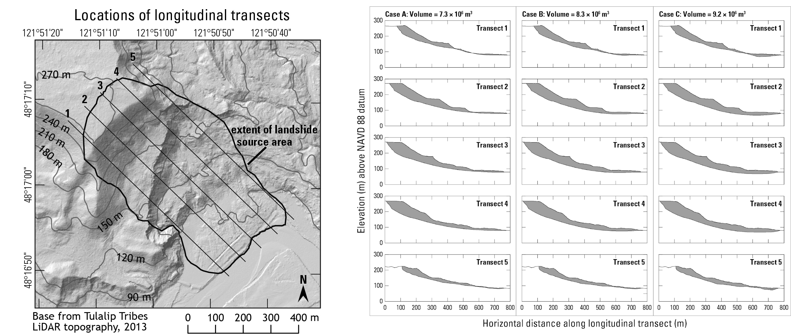
Estimation of the total volume of the Oso landslide required differencing the 2013 and 2014 lidar topography, but also required reconstruction of the landslide’s basal slip-surface geometry. This reconstruction was necessary because considerable landslide debris remained in the source area at the conclusion of the event. Three alternative reconstructions yielded source-area volume estimates ranging from 7-9 million cubic meters, with the intermediate volume deemed most plausible (Iverson et al., 2015). This basal slip surface reconstruction, along with the 2013 lidar topography, also established the initial geometry used in the model simulations presented here.
Using D-Claw to reveal landslide mobility bifurcations based on material parameters
The evolution of material strength in a landslide that liquefies is contingent on the evolving dynamics of the landslide as a whole. Therefore, realistic models of liquefying landslides cannot be founded on traditional rheological formulas, which specify that local resistance to motion is a function of only local stress states and displacements or displacement rates (Iverson, 2003). Instead, realistic models must allow the apparent rheology to evolve in response to feedbacks that develop as the distributions of landslide mass, momentum and pore pressure evolve. These large-scale feedbacks can cause time- and space-dependent changes in the local material state, similar to changes that play a central role in quasi-static, critical-state soil mechanics. In contrast to evolving material states in quasi-static soils, however, evolving material states in liquefying landslides may be influenced by arbitrarily large, rapid displacements and momentum transfer.
Models that aim to explain the behaviour of landslides that liquefy must also be able to explain landslide behaviour in which liquefaction does not occur – without invoking differences in intrinsic granular friction. Models that lack this discriminatory power can shed no light on factors favouring or limiting the potential for liquefaction and attendant high mobility. Indeed, the difference between relatively slow, stable landslide motion and unstable, liquefying landslide motion may represent a sharp behavioural bifurcation (Iverson et al., 2000; Iverson, 2005). Important questions about such a bifurcation concern its sensitivity to initial conditions and material properties.

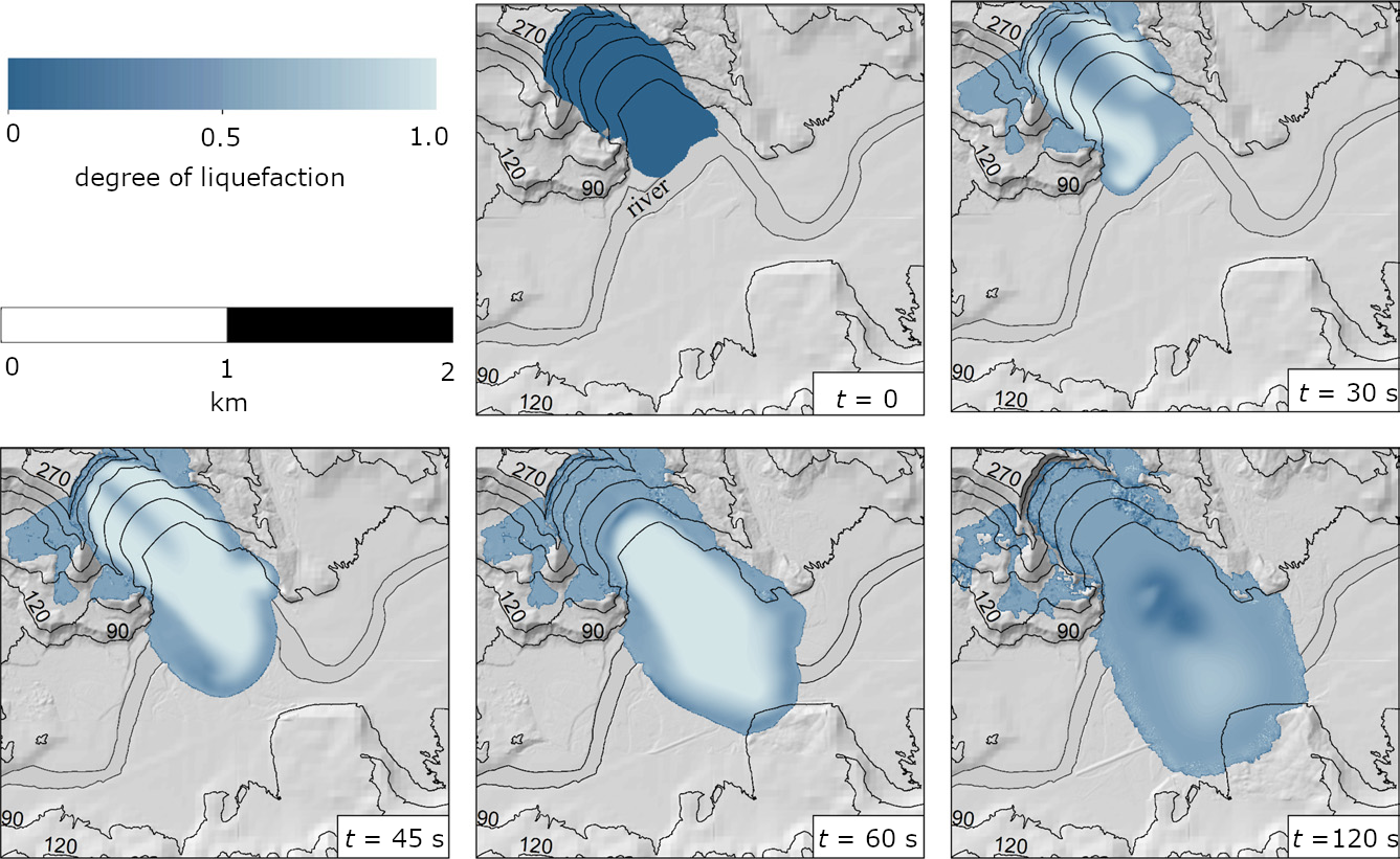
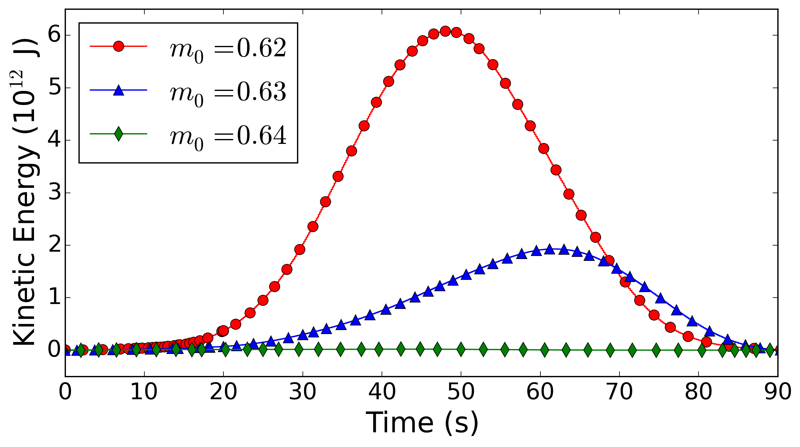
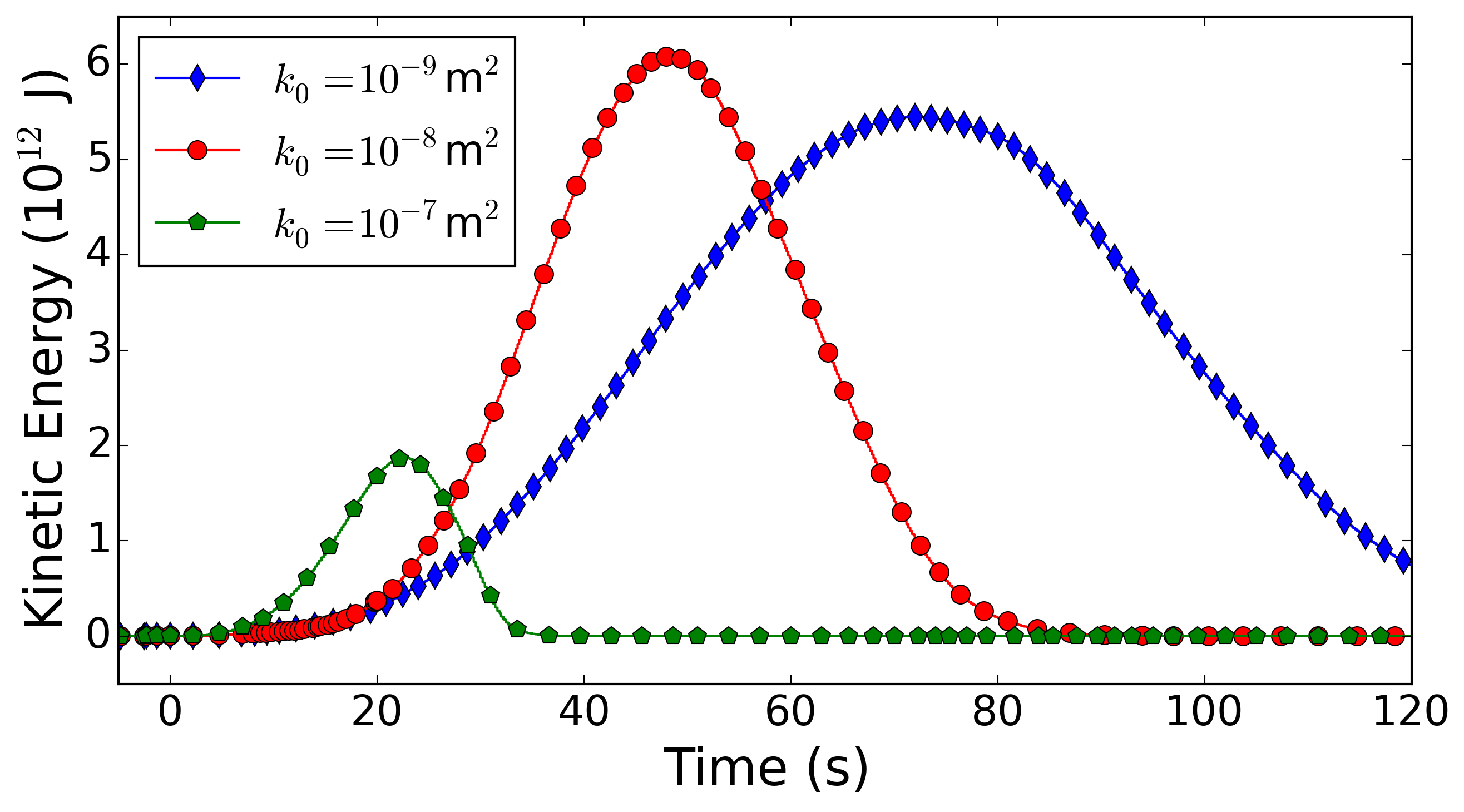
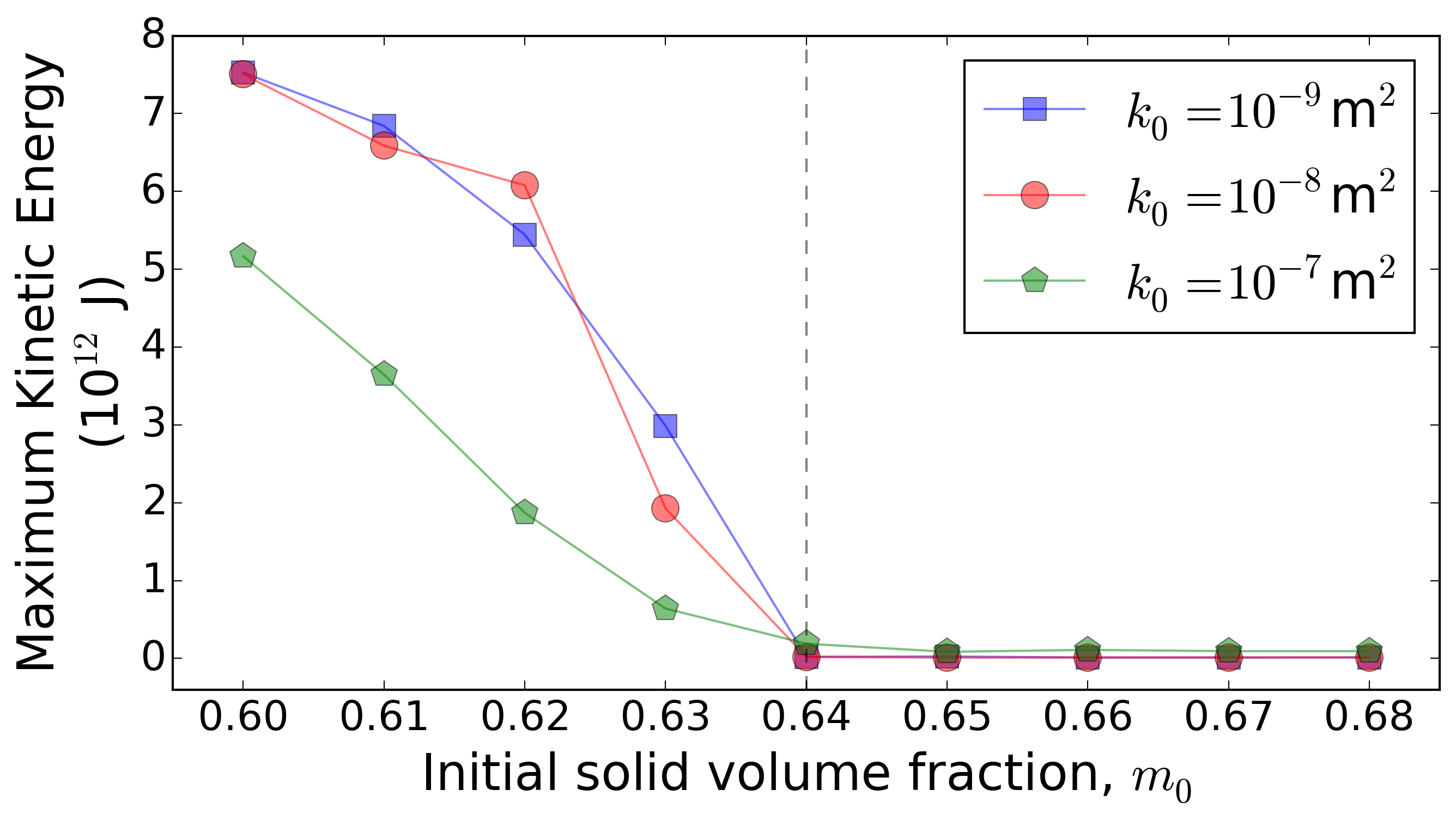
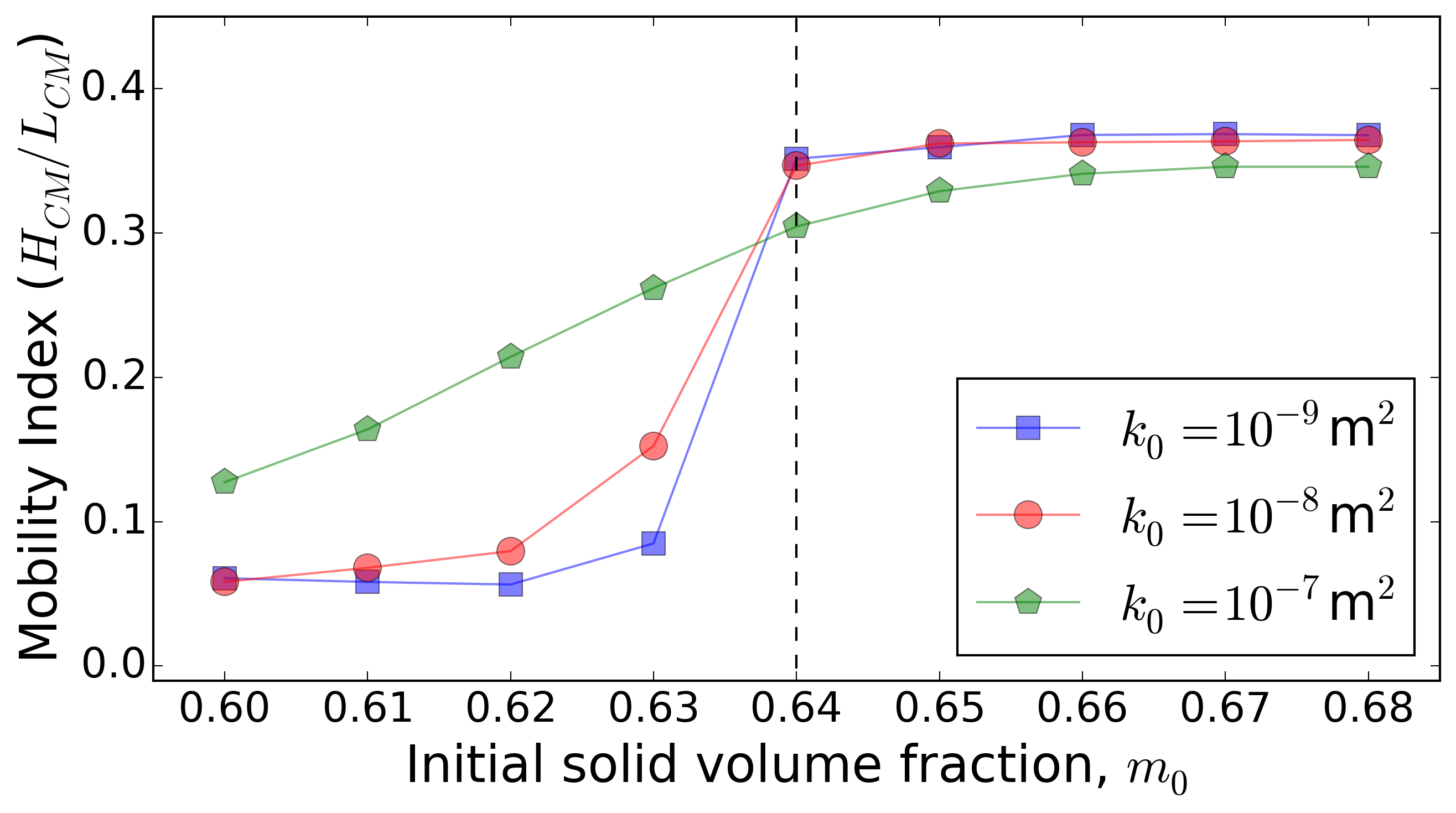
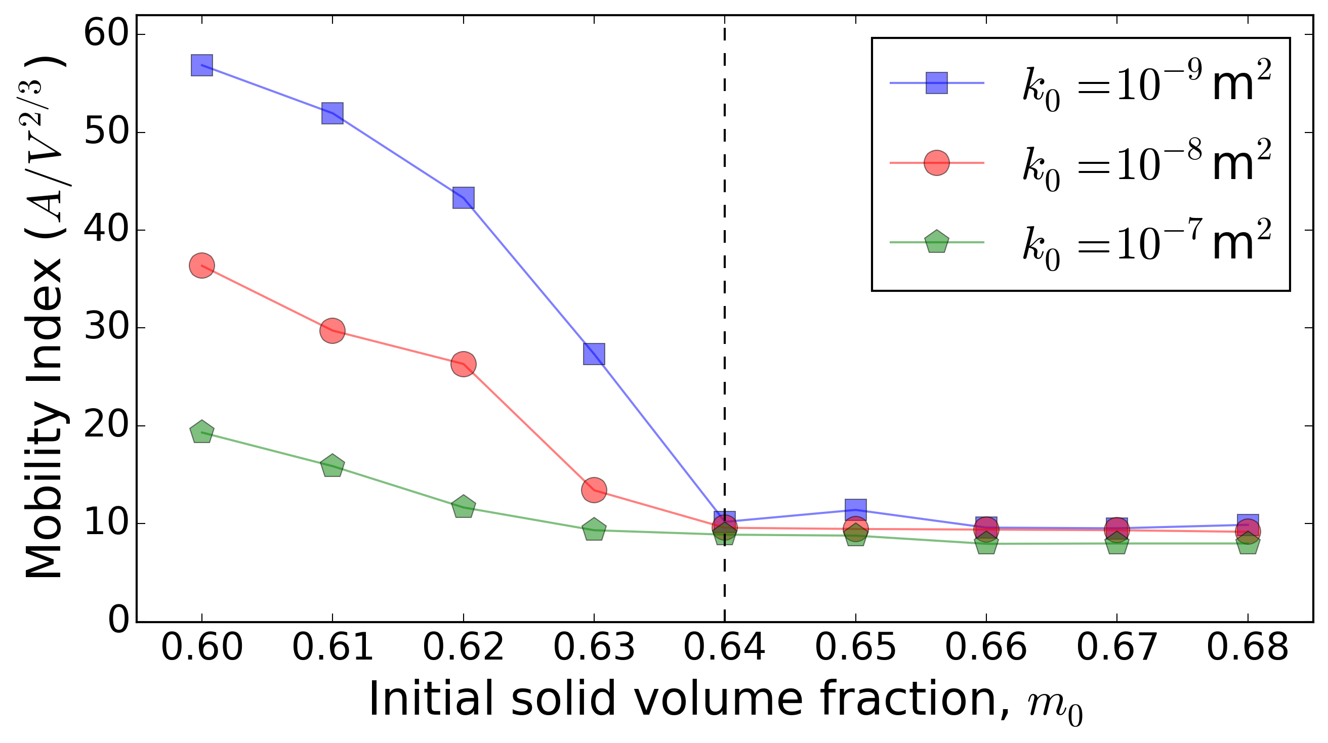
Here the focus is placed on insights that can be gained from using D-Claw to model the dynamics of the landslide as well as a spectrum of alternative behaviours computed for landslides with the same initial geometry and basal friction angle, but with modified values of the initial solid volume fraction m0 and permeability k0.
Conclusions
An important practical implication of these findings is that large differences in landside mobility can result from small differences in initial conditions. Model studies aimed at landslide hazard prognostication can in principle account for the associated uncertainties by adopting probabilistic methods. Nevertheless, the challenge in making useful predictions is great, because bifurcating landslide dynamics can result in divergent outcomes.
References
- Landslides that liquefy: modeling mobility bifurcation and the 2014 Oso, Washington, USA disaster. R.M. Iverson, D.L. George, 2016. Geotechnique, V. 66(3), 175–187. pdf
- Landslide mobility and hazards: implications of the 2014 Oso disaster. R.M. Iverson, D.L. George, et al., 2015. Earth Planet. Sci. Lett., V. 412, pp. 197–208. pdf
- A depth-averaged debris-flow model that includes the effects of evolving dilatancy: 2. Numerical predictions and experimental tests. D. L. George and R.M. Iverson, 2014. Proc. R. Soc. A, 470 (2170). pdf
- A depth-averaged debris-flow model that includes the effects of evolving dilatancy: 1. Physical basis. R.M. Iverson and D.L. George, 2014. Proc. R. Soc. A, 470 (2170). pdf