Modeling a large landslide near Tyndall Glacier and the resulting tsunami in Taan Fjord, Alaska
This page features excerpts and figures from:
New methodology for computing tsunami generation by subaerial landslides: application to the 2015 Tyndall Glacier Landslide, Alaska. D. L. George, R.M. Iverson and C.M. Cannon, 2017. Geophys. Res. Lett., V. 44(14), 7276–7284. pdf.
Abstract
Landslide-generated tsunamis pose significant hazards and involve complex, multiphase physics that are challenging to model. We present a new methodology in which our depth-averaged two-phase model D-Claw is used to seamlessly simulate all stages of landslide dynamics as well as tsunami generation, propagation, and inundation. Because the model describes the evolution of solid and fluid volume fractions, it treats both landslides and tsunamis as special cases of a more general class of phenomena. Therefore, the landslide and tsunami can be efficiently simulated as a single-layer continuum with evolving solid-grain concentrations, and with wave generation via direct longitudinal momentum transfer—a dominant physical mechanism that has not been previously addressed in this manner. To test our methodology, we used D-Claw to model a large subaerial landslide and resulting tsunami that occurred on 17 October 2015, in Taan Fjord near the terminus of Tyndall Glacier, Alaska. Modeled shoreline inundation patterns compare well with those observed in satellite imagery.
Introduction
Coseismic tsunamis such as the 2004 Indian Ocean and 2011 Tohoku tsunamis have widespread impacts, but subaerial landslides that enter water bodies can produce equally destructive waves, albeit at more localized scales. Examples include the 1958 Lituya Bay, Alaska, rockslide (≈ 30 million cubic meters) and tsunami, which resulted in the highest known inundation in historical times (≈ 525 m) [Miller, 1960; Fritz et al., 2001], and more recently, the 2015 Tyndall Glacier, Alaska, landslide (70–80 million cubic meters) [Stark, 2015] and resulting Taan Fjord tsunami. Efficient, accurate, robust models are needed to understand the physics of landslide-generated tsunamis and to assess the associated hazards.
Landslide-generated tsunamis present unique modeling challenges because of the need to compute landslide dynamics as well as wave-generation and wave-propagation dynamics. Here we propose using single-layer, multiphase, depth-averaged model to seamlessly simulate all stages of subaerial landsliding and consequent tsunami generation and propagation. In this model momentum conservation and exchange occurs naturally as the landslide material interacts with the water body and generates impulse waves. We test our approach by comparing model predictions with tsunami inundation limits observed in satellite imagery, and we also compare our predictions with results obtained using a more traditional methodology.
The 2015 Tyndall Glacier landslide and tsunami, Taan Fjord, Alaska.
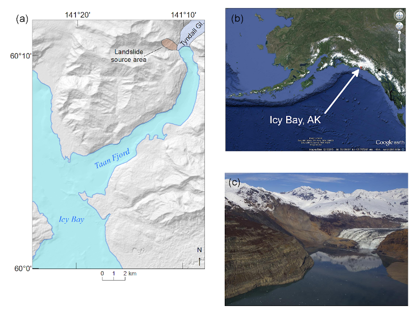
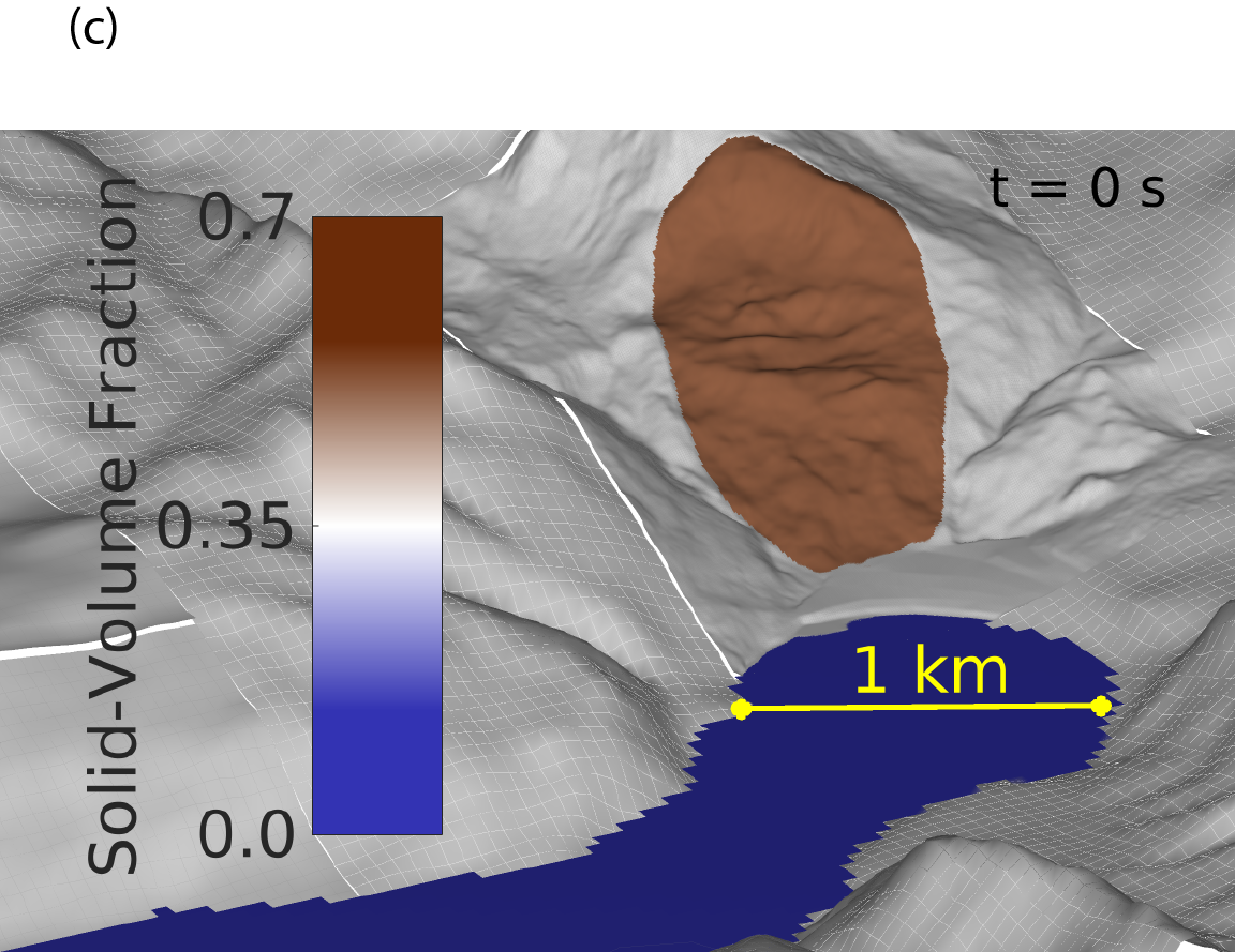
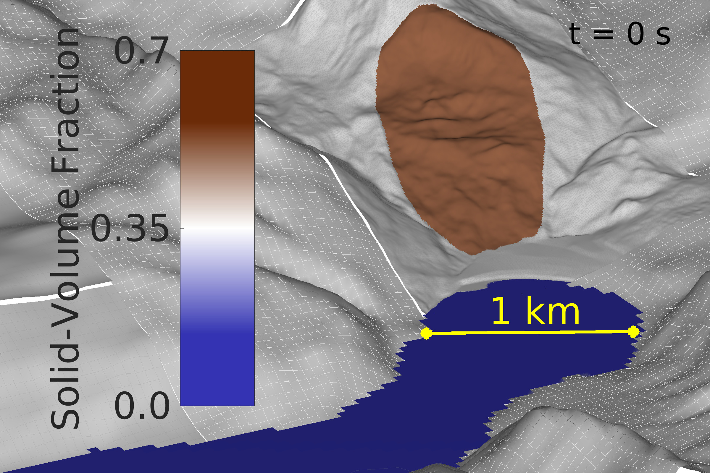
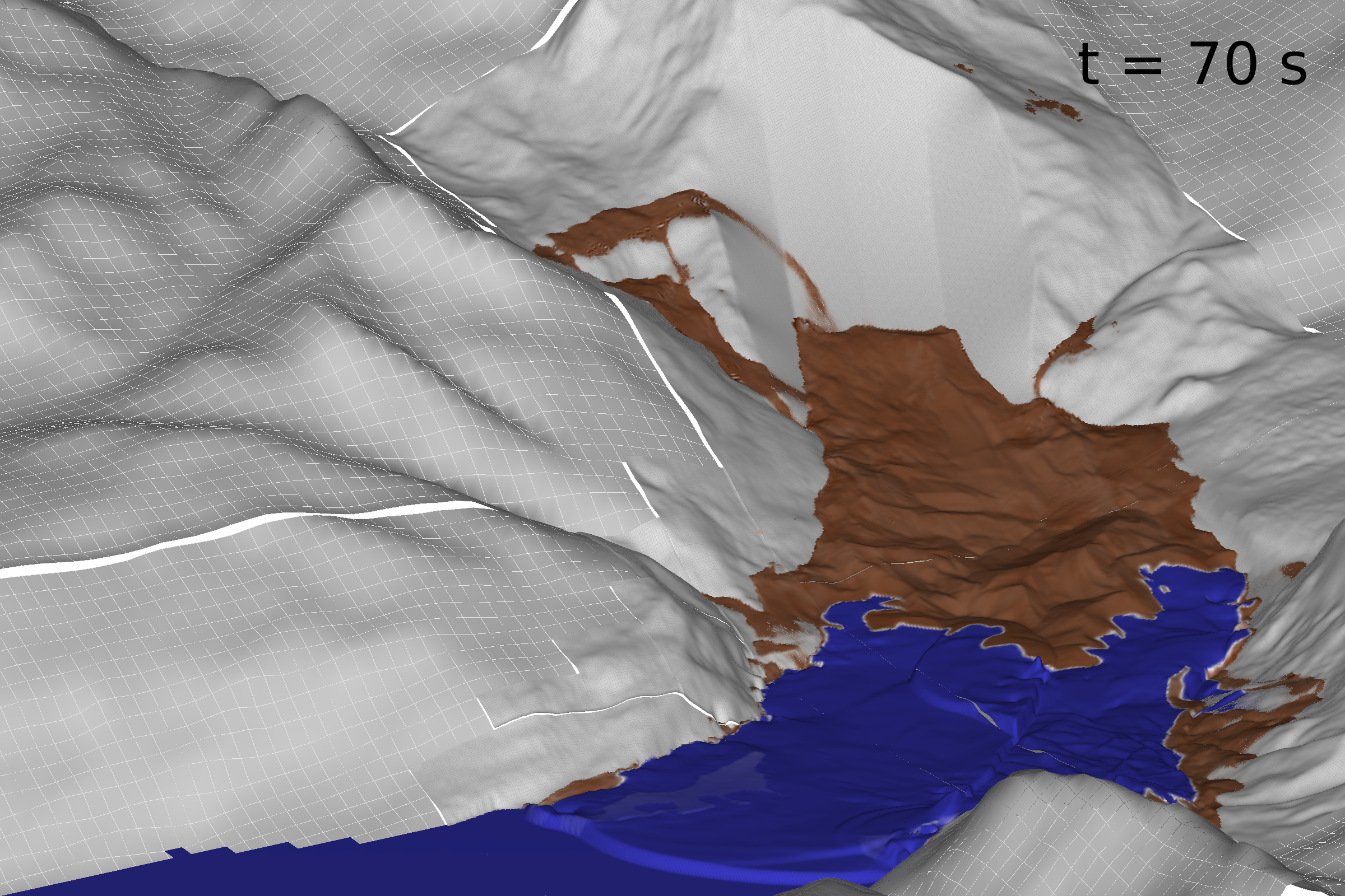
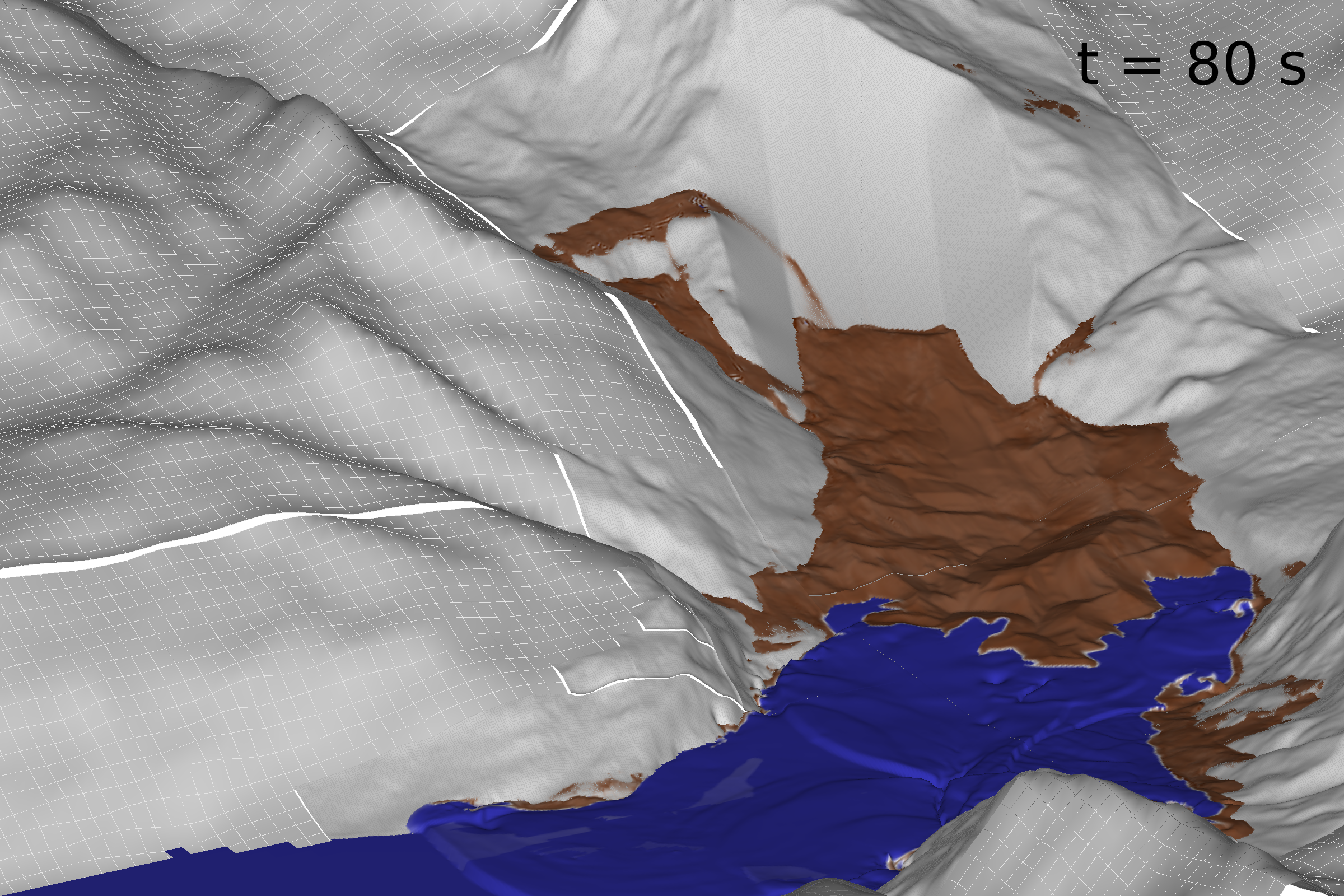
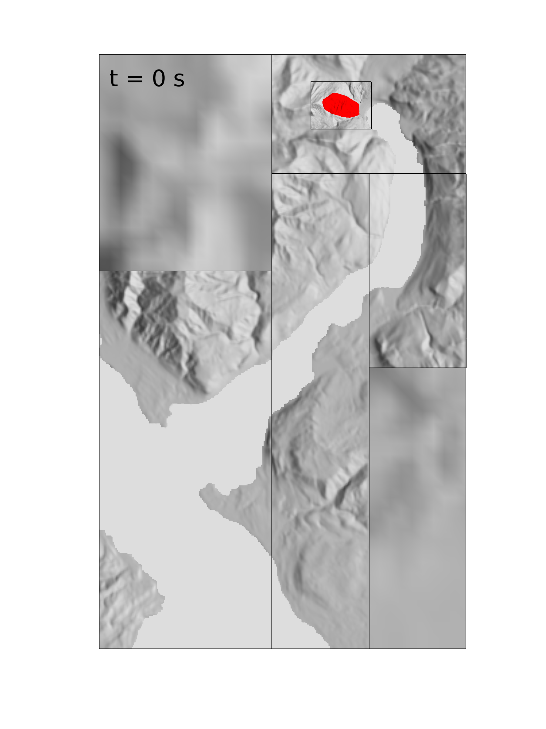
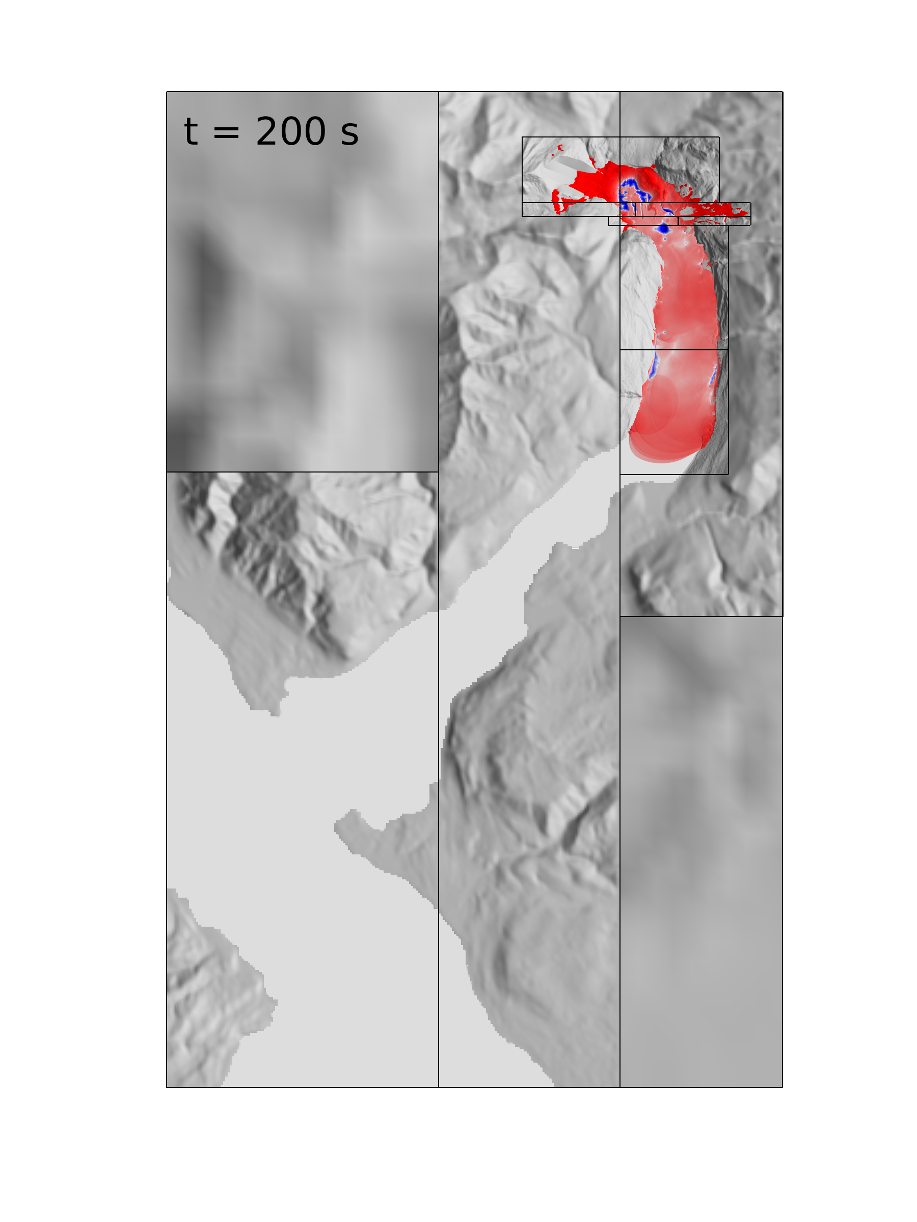
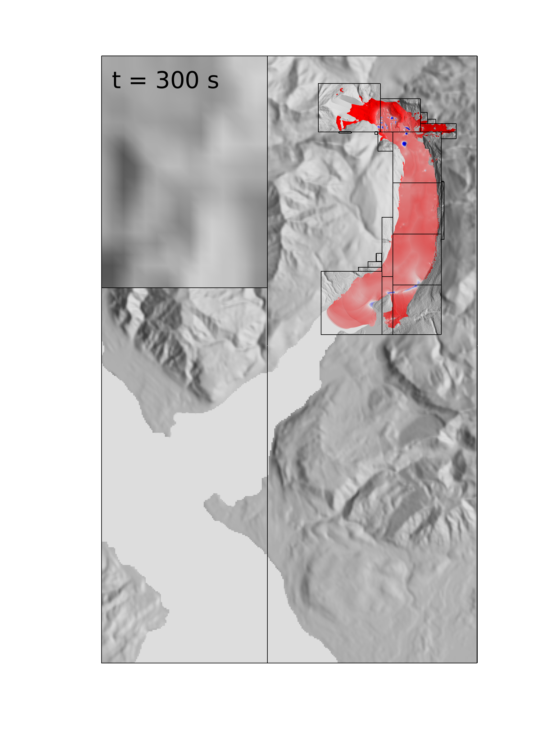
At about 8:19 P.M. (local time) on 17 October 2015, after a period of heavy rain, a large landslide occurred near the toe of Tyndall Glacier, which originates on the flanks of Mount St. Elias and terminates at the head of Taan Fjord and Icy Bay, Alaska (Figure 1). Runout of the 2015 landslide generated a tsunami in Taan Fjord that reached vertically 150 m up a hillside on the opposite side of the fjord (Rozell, 2016). Landslide mass estimates from the long-period seismicity radiated by the landslide were about 180 billion kg, which implies a volume of about 70–80 million cubic meters (Stark, 2015).
Modeling the landslide and tsunami with D-Claw
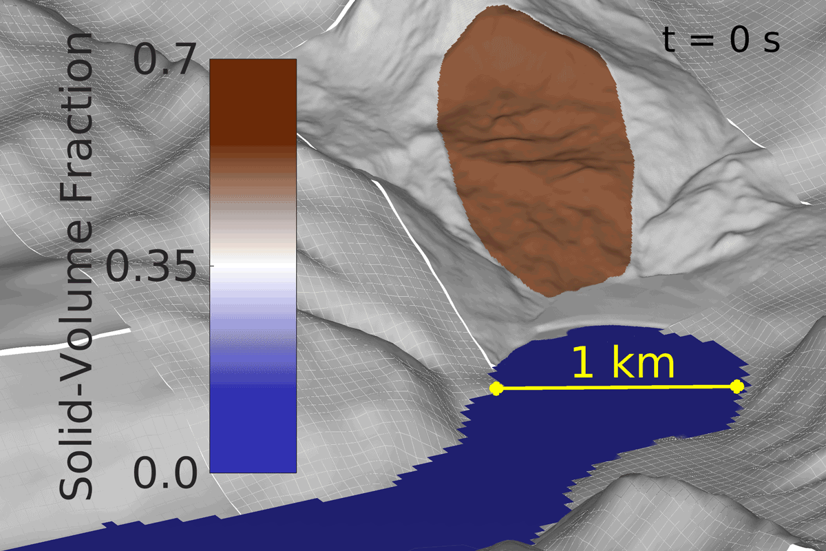
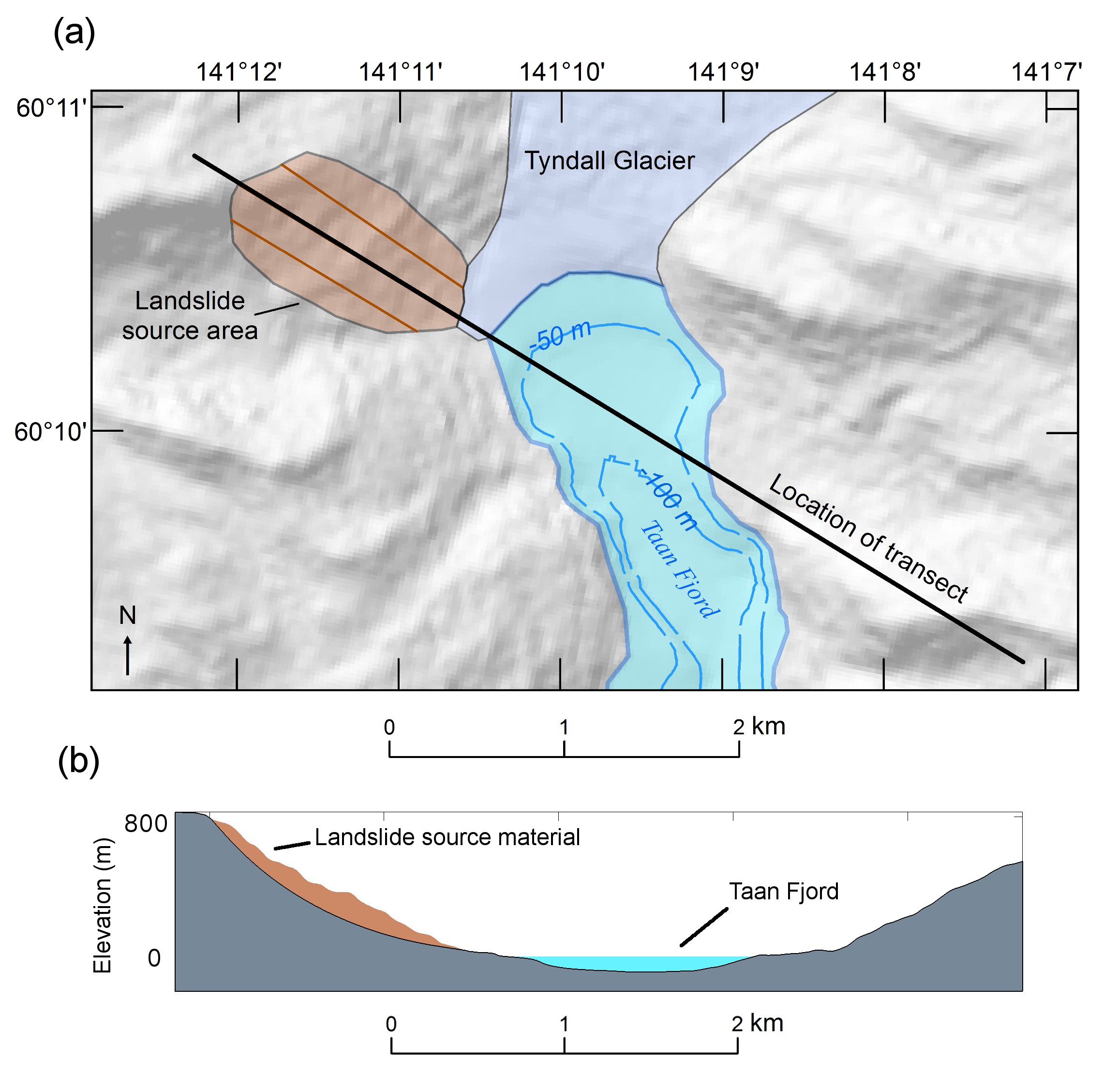
We outlined the 2015 landslide source area extent by interpreting satellite topography and imagery of the older slump deposit at the site. We approximated the landslide basal slip surface by fitting logarithmic spirals along three longitudinal transects drawn orthogonal to scarps within the landslide (Figure 2). (In lieu of additional data, landslide slip-surface profiles are commonly assumed to have log-spiral shapes.) The logarithmic spirals were constrained by the inferred scarp and toe inclinations, and by the landslide volume estimate of 70–80 million cubic meters. The consequent modeled landslide source area is 0.9 square kilometers and volume is 78 million cubic meters.
 "
"
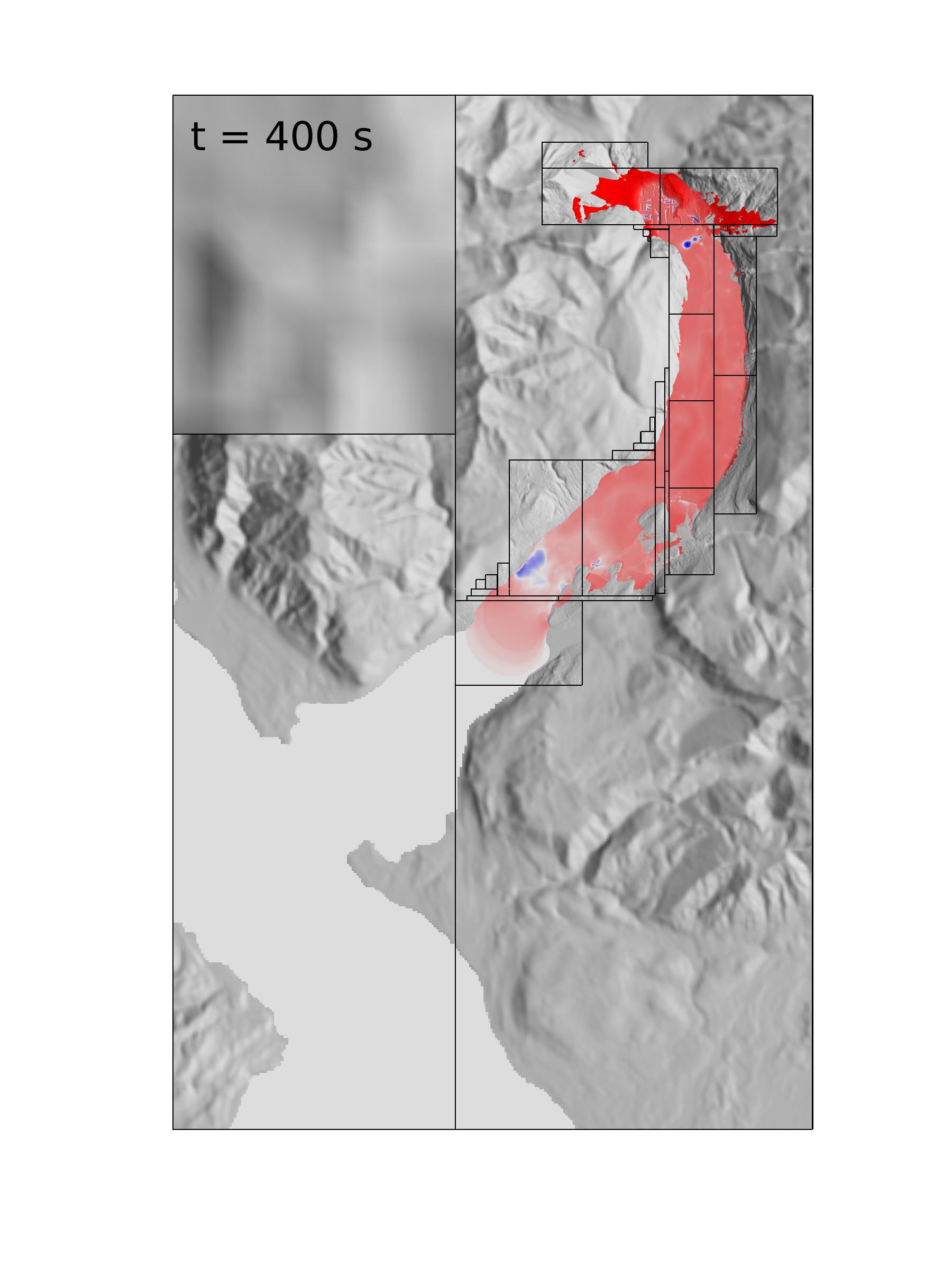
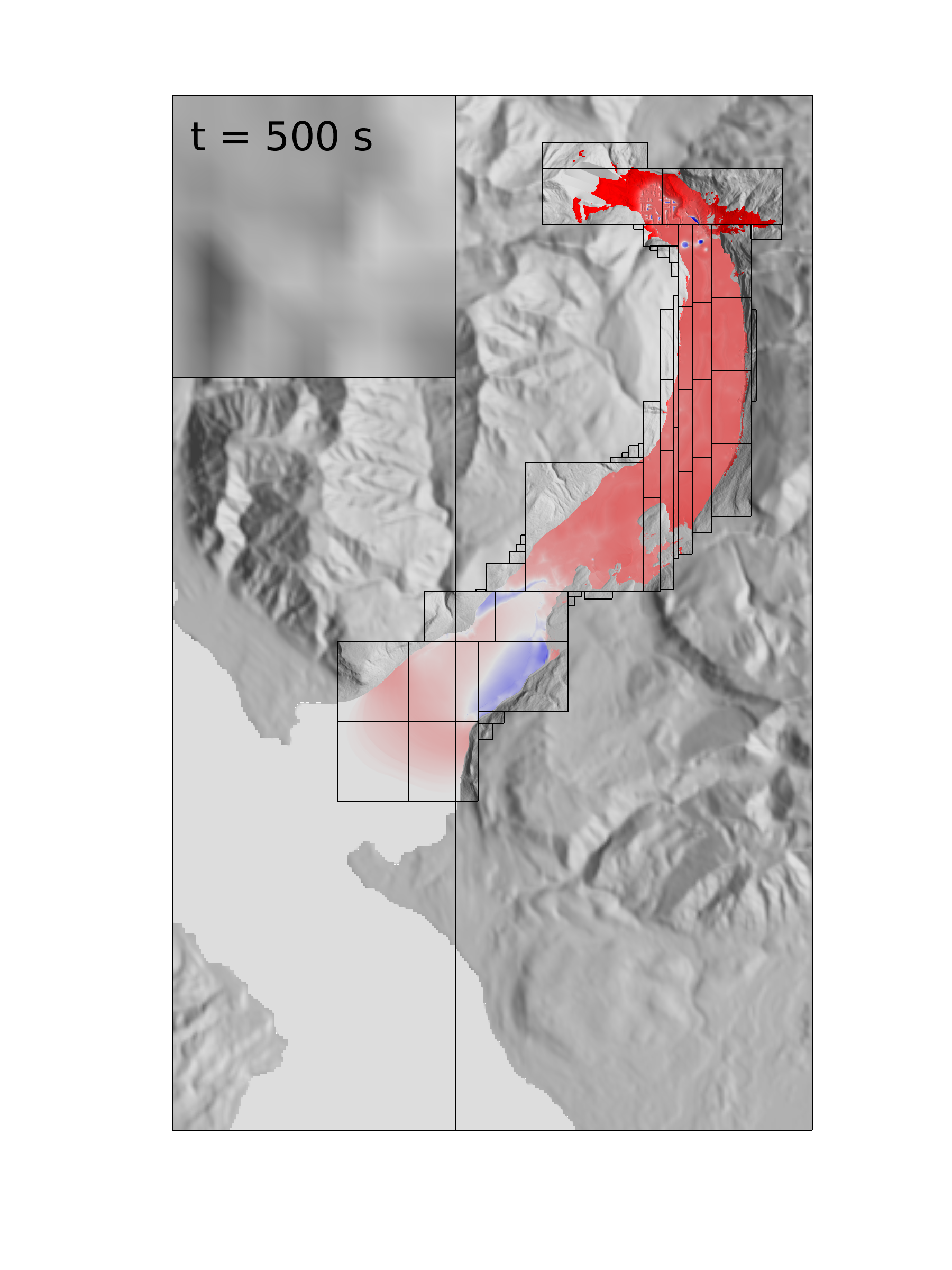
With our hypothetical landslide source models we simulated landslides, tsunami generation, wave propagation, and inundation along Taan Fjord with several methodologies including D-Claw. To model tsunamis generated by subaerial landslides, we initialize D-Claw by representing the landslide source material as a statically balanced, homogeneous grain-water mixture, and by representing the water body as a static pure fluid. Impulse waves are generated naturally as the denser landslide mixture impacts the water body and exchanges mass and momentum with it.
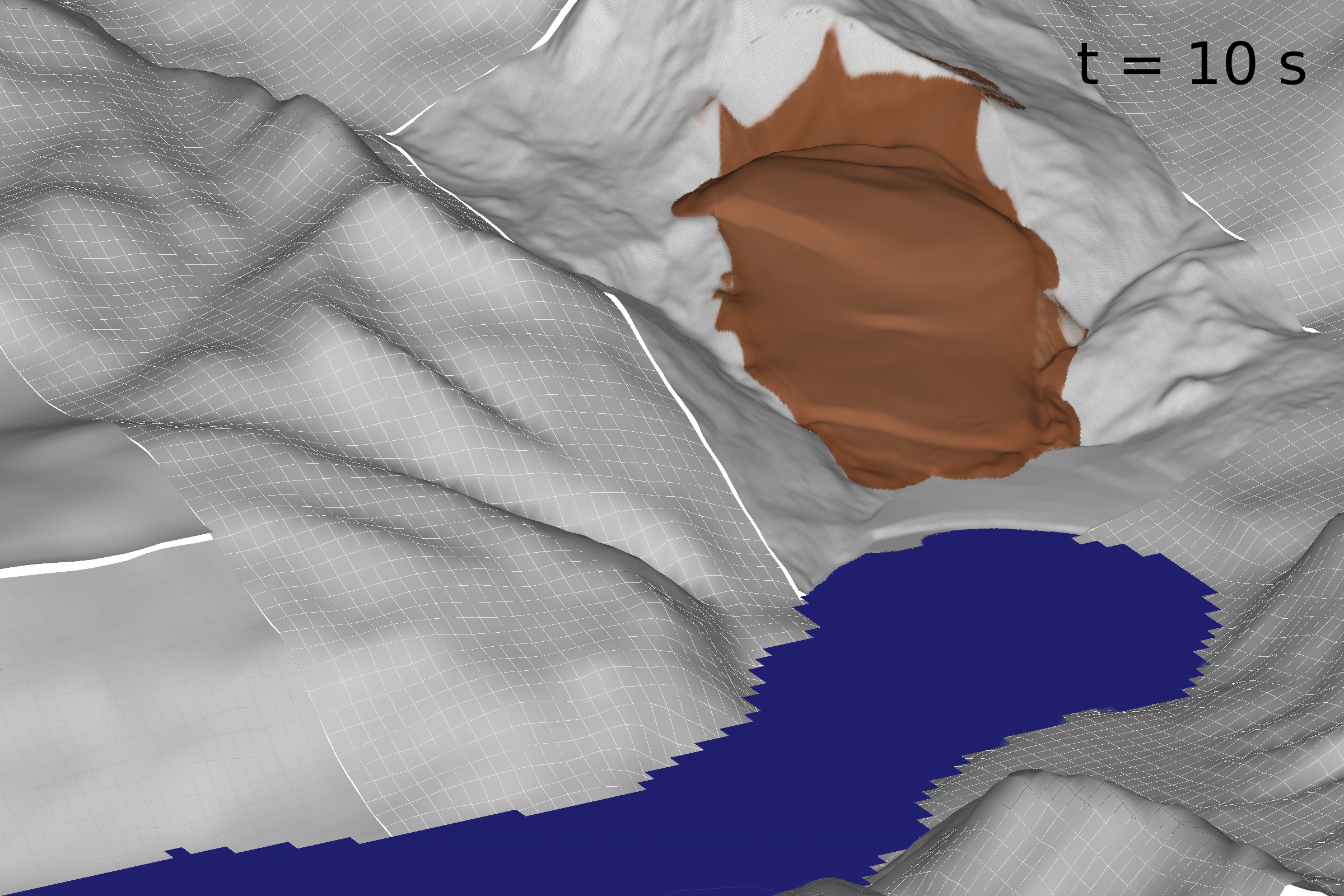
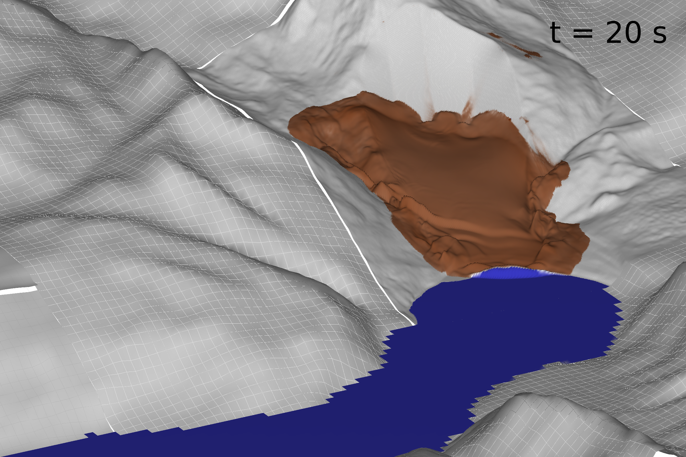
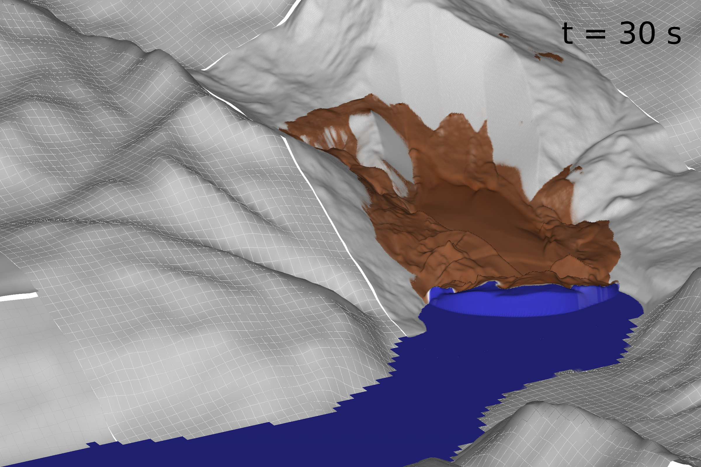
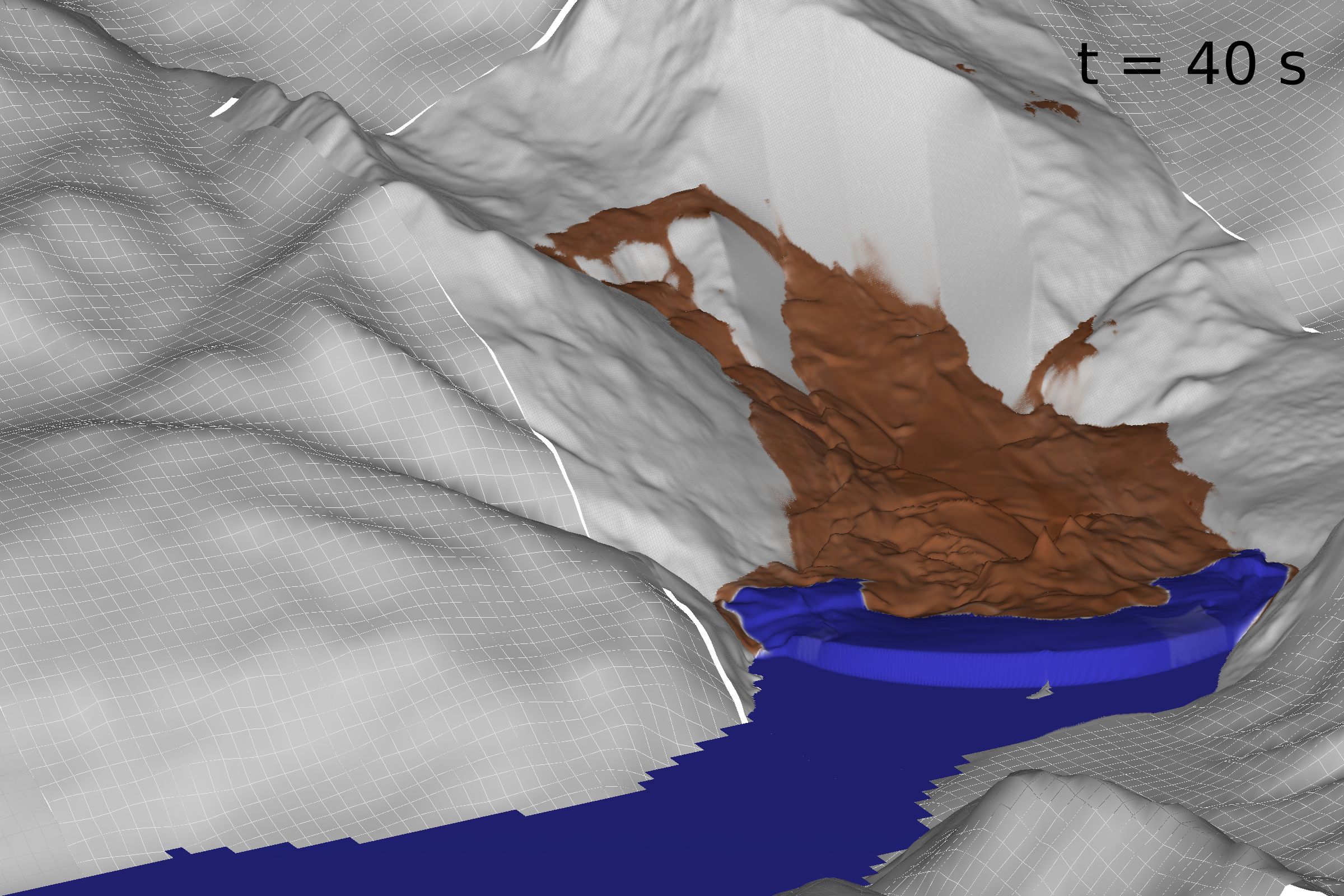
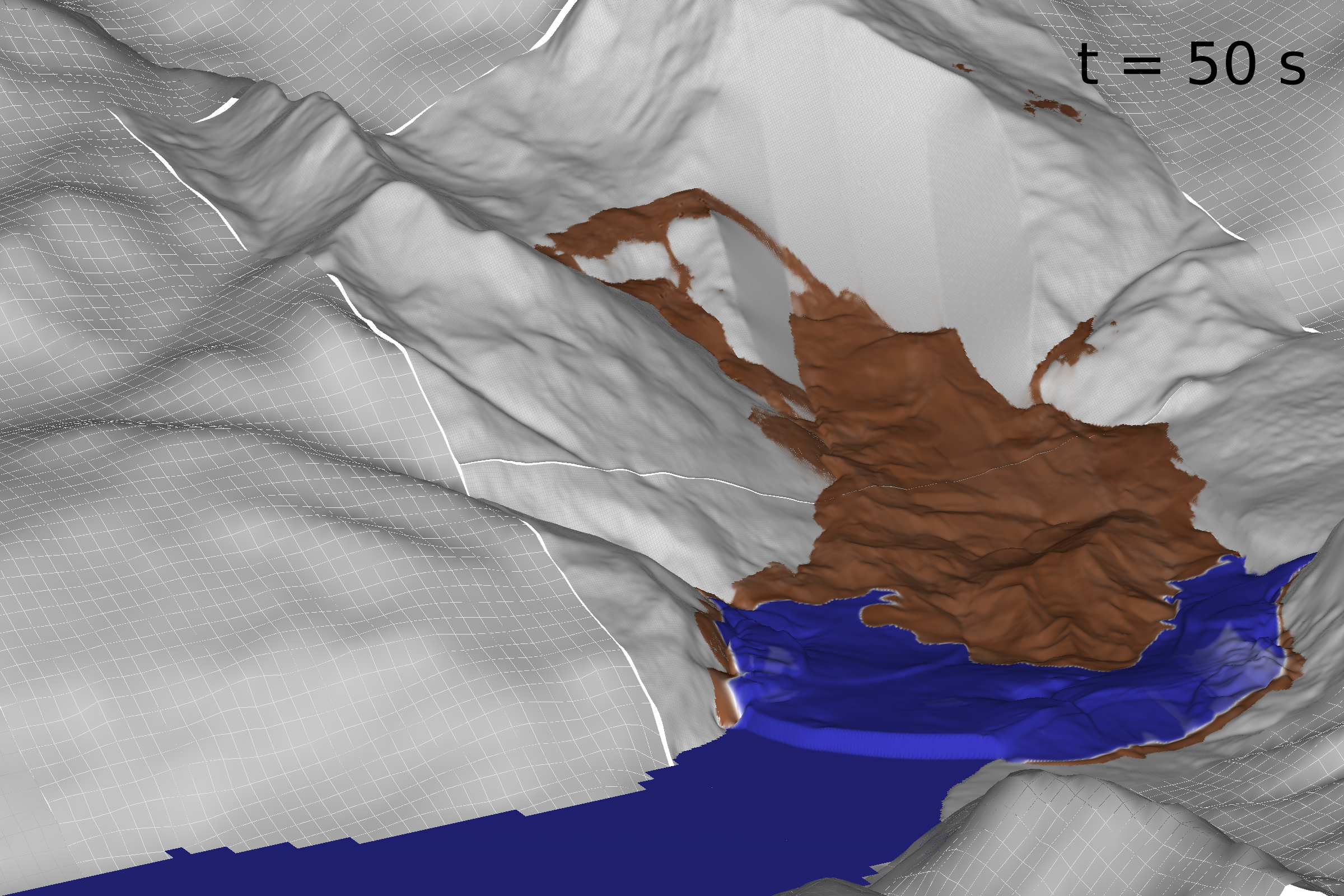
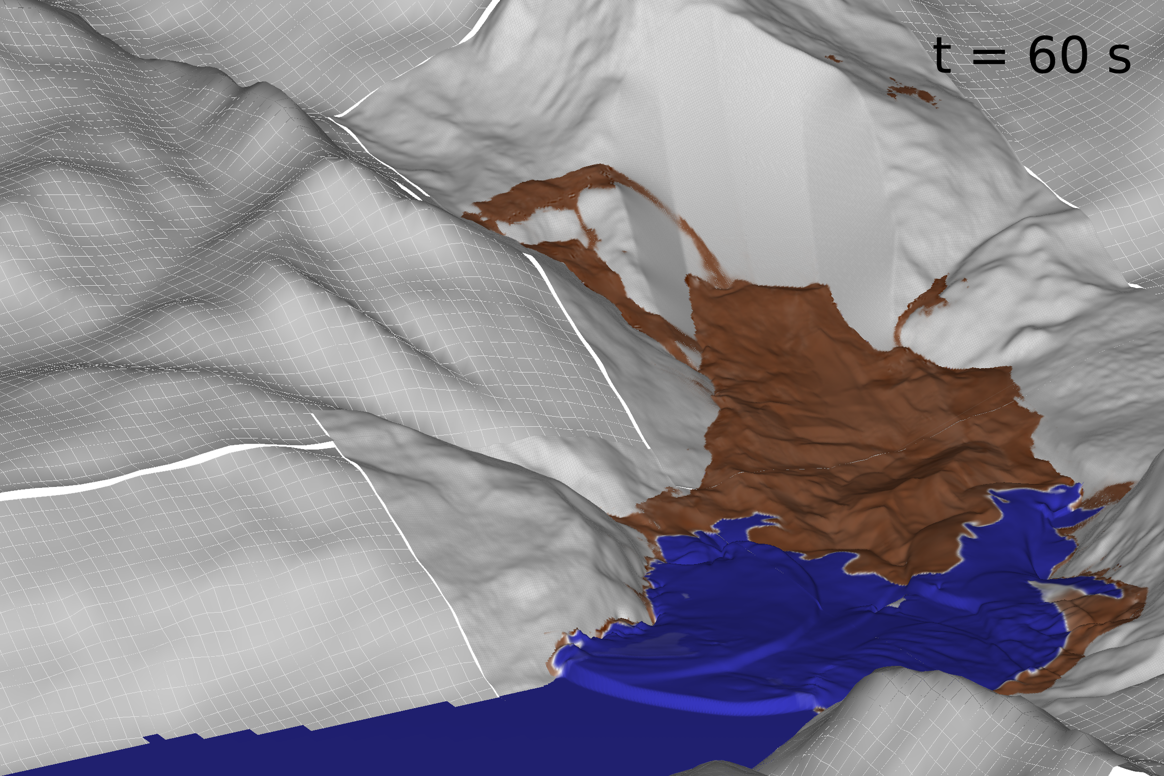
A key advantage of this approach is that it does not require specification of coupling mechanisms to link distinct models for landslide motion, wave generation, and wave propagation. If the depth and length scales of the landslide and impacted water body are similar (Figure 2), then the shallowness assumption used to derive the D-Claw equations can be applied to the entire continuum as a single layer—as is commonly done for modeling landslides and tsunamis individually. If the impacted water body is deep relative to the landslide mass, then the single-layer assumption becomes more tenuous and multiple layers that exchange mass and momentum might be warranted.
Comparison of modeling approaches and data
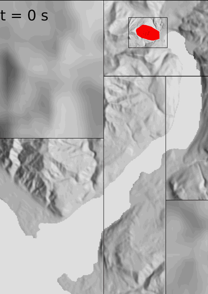
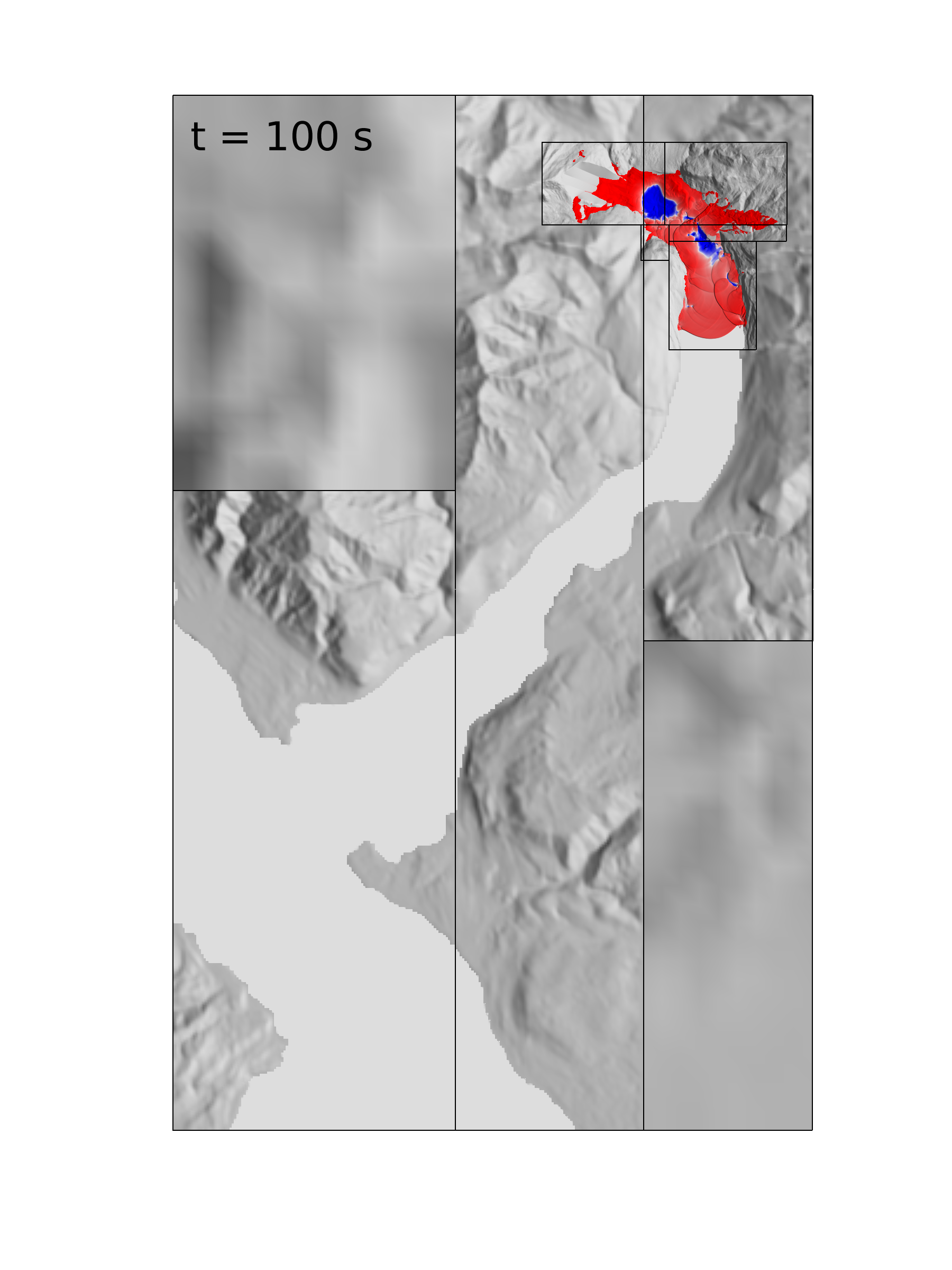
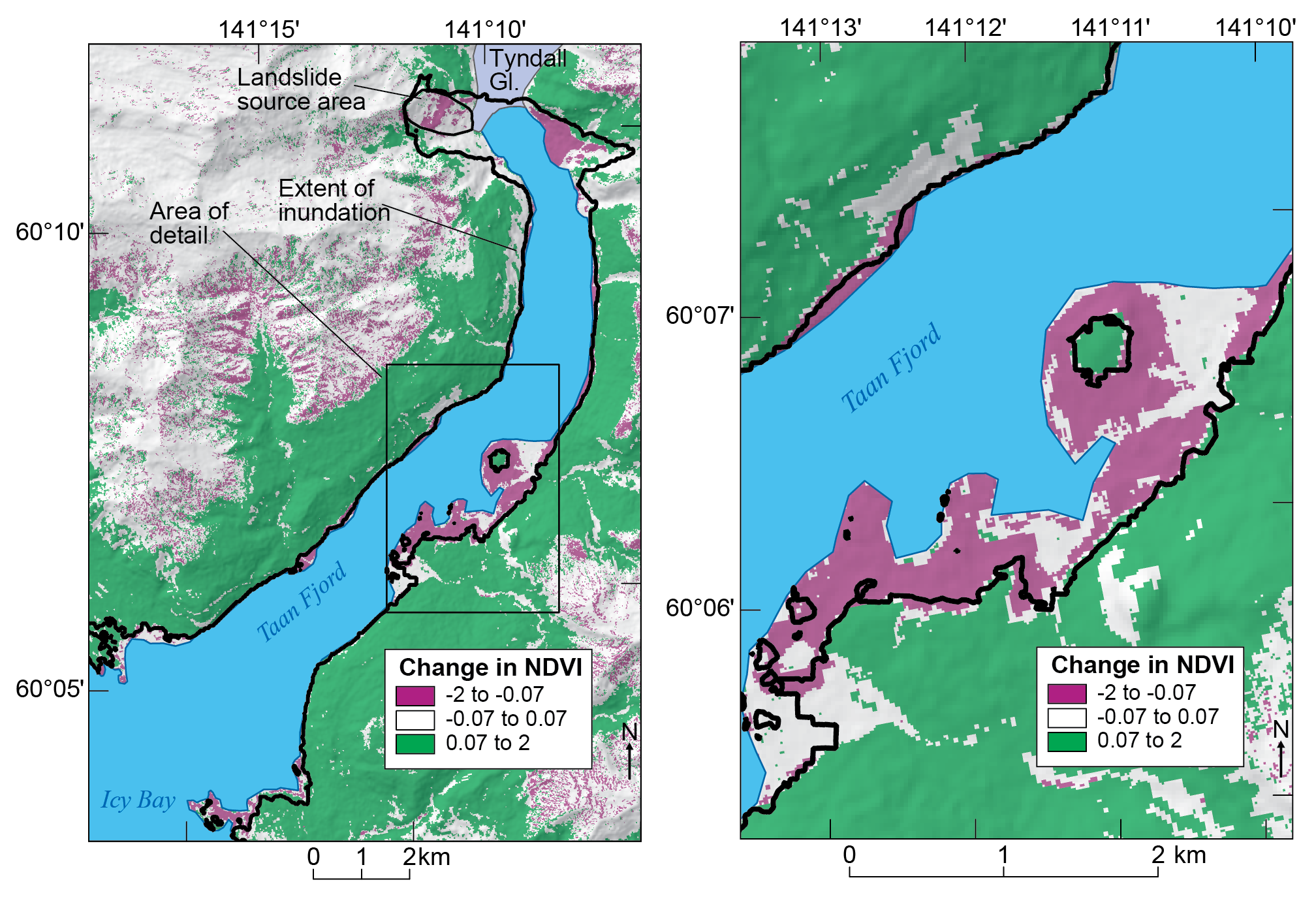
We utilized satellite imagery to compare observed tsunami inundation limits with those predicted . Aerial imagery taken after the tsunami shows clear signs of inundation and vegetation removal along the shores of Taan Fjord [Rozell, 2016]. We used pan-sharpened Landsat 8 Operational Land Imager images from 14 May 2015 and 15 May 2016 to assess vegetation change. NDVI results from 2015 were subtracted from results for 2016 to produce a change image shown in Figure 7. Overall, there is more vigorous vegetation growth in the Taan Fjord area in 2016, but there are conspicuous areas of vegetation removal adjacent to the shoreline. The extent of inundation predicted by the seamless D-Claw simulation is outlined in black in Figure 7.
To help evaluate the results obtained using our new methodology, we also performed more traditional simulations in which we first precomputed the landslide dynamics in the absence of water and then used the computed landslide surface as an evolving basal boundary surface for simulating tsunami generation and propagation (Figure 8). The same model parameters were used for all simulations.
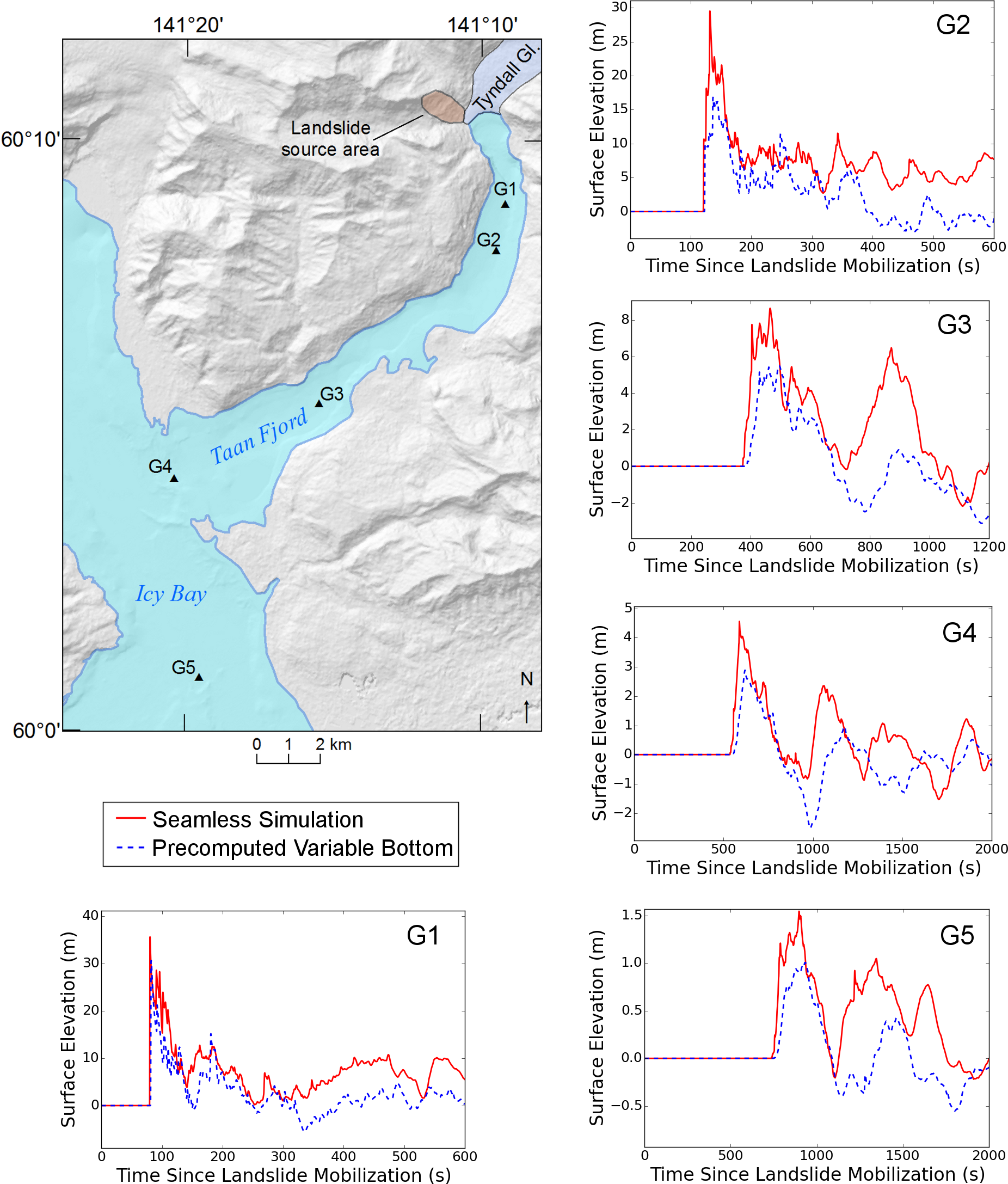
Figure 6 compares results generated by using our new methodology and the more conventional and more labor-intensive boundary-displacement methodology to compute time series of water waves at five locations in Taan Fjord and Icy Bay. Given the dramatically different assumptions about wave generation processes in these alternative approaches, broadly similar tsunami waves are predicted at points distant from the landslide. The seamless D-Claw simulation produces a larger peak amplitude, however—particularly near the source area—and it involves no user intervention to create evolving boundary conditions.
Conclusions
Our seamless D-Clawsimulations of the Tyndall Glacier landslide and Taan Fjord tsunami used an uncalibrated model but produced shoreline inundation patterns that are consistent with the data currently available.More in-depth comparisons would require higher-resolution bathymetry and topography as well as additional field data. Comparisons of two alternative approaches (seamless versus precomputed landslide and evolving seafloor) predict similar tsunami waves in Taan Fjord and Icy Bay. Thus, the two approaches would likely lead to similar assessments of inundation hazards in this particular case. However, the seamless approach using D-Claw has clear computational and methodological advantages because it avoids the step of precomputing an evolving spatiotemporal landslide surface, and the mass and momentum of the system are automatically resolved owing to the absence of quasi-coupled model interfaces. Our results suggest that D-Claw can simulate the impulse waves associated with subaerial landslide tsunamis with sufficient fidelity for hazard forecasting.
References
- Rozell, N. (2016), The Giant Wave of Icy Bay, Geophys. Inst. AK Press Release, Fairbanks, Alaska. Available at www.gi.alaska.edu/alaska-science-forum/giant-wave-icy-bay.
- Stark, C. P. (2015), Landslide dynamics from seismology: New results, Abstract EP51D-08 presented at 2015 Fall Meeting, AGU, San Francisco.